String Method for Minimum Free Energy Paths

📋 Tutorial Summary
Learn the string method for finding minimum free-energy paths (MFEPs) between metastable states in a low-dimensional collective-variable (CV) space. Includes a toy Python implementation on the Müller–Brown potential.

Overview

The string method constructs a path between two states (A → B) as a set of discrete images (“beads”) in CV space, then iteratively updates the path so it aligns with the local free-energy landscape (approaches the MFEP). Conceptually it is closely related to elastic-band approaches (e.g., NEB), but formulated in collective-variable space and typically driven by mean forces rather than a simple potential-energy gradient.

You’ll typically use it when:

You have two metastable basins and want the most likely transition pathway.
Direct sampling of transitions is rare (high barriers / timescales not accessible with standard simulation).
You can define a small set of CVs that capture the mechanism.

Direct simulation can be very inefficient for rare events. You can see that here:

Overdamped Langevin trajectory (1000 steps) on the Müller–Brown potential — Overdamped Langevin trajectory example (1000 steps) started in basin A.This is a Langevin simulation on a potential energy surface where the trajectory is initialized in one stable basin. It would be quite inefficient to run unbiased dynamics until you generate a statistically significant set of transition pathways between two states.

References

There are many flavors of the string method (mean-force, swarm-of-trajectories, finite-temperature strings, etc.). Two useful references:

E, Ren, Vanden-Eijnden (2002) — “string method for the study of rare events” (PhysRevB.66.052301)
Maragliano, Roux, Vanden-Eijnden (2014) — comparison between mean-force and swarm-of-trajectories string methods (PMC6980172)

These methods are related to older elastic-band / reaction-path ideas developed decades ago. For example:

Elber, Karplus (1987) — “A method for determining reaction paths in large molecules: Application to myoglobin” (ScienceDirect)

It’s a classic paper. The paper shows that many of the core ideas inrepresenting a transition as a discretized path and iteratively refining it, were already being explored in the 1980s when MD was just starting to take off. The method they proposed had some artificats that subsequent adjustments were made to get the Nudged Elastic Band that is commonly used in Quantum Mechanical Calculations.

High-level algorithm

Choose CVs and define endpoints (A and B) in CV space. (CV choice is the hard part.)
Initialize a string: a set of images between A and B (linear interpolation is common).
For each image, estimate the mean force (e.g., by restrained sampling / umbrella windows).
Update the string by moving images along the mean force (typically projected normal to the string).
Reparameterize the string (redistribute images to keep roughly uniform spacing).
Iterate until the string stops changing within tolerance.

Minimal pseudo-code

initialize images s_i (i=1..N) from A to B
repeat until converged:
  for each image i:
    run restrained sampling at s_i
    estimate drift v_i  (e.g., mean force direction)
    s_i <- s_i + dt * v_i
  reparameterize {s_i} to enforce uniform arc-length spacing

Toy example: Müller–Brown potential

This page includes a toy 2D string-method demo implemented in:

tutorials/string_method/string_method_test.py

It uses the classic Müller–Brown potential energy surface:

\[V(x,y) = \sum_{i=1}^{4} A_i \exp\left[a_i(x-x_i)^2 + b_i(x-x_i)(y-y_i) + c_i(y-y_i)^2\right]\]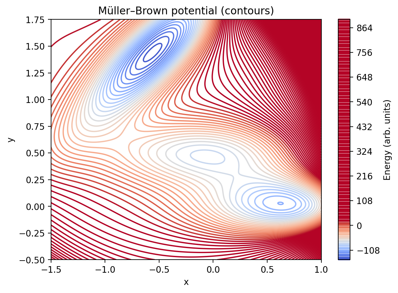

Müller–Brown potential energy surface (contours) — Müller–Brown potential (contour plot).

with the standard parameter set:

A  = [-200, -100, -170, 15]
b  = [0, 0, 11, 0.6]
x0 = [1, 0, -0.5, -1]
a  = [-1, -1, -6.5, 0.7]
c  = [-10, -10, -6.5, 0.7]
y0 = [0, 0.5, 1.5, 1]

What the demo does (conceptually)

Build and plot the potential energy surface (contours).
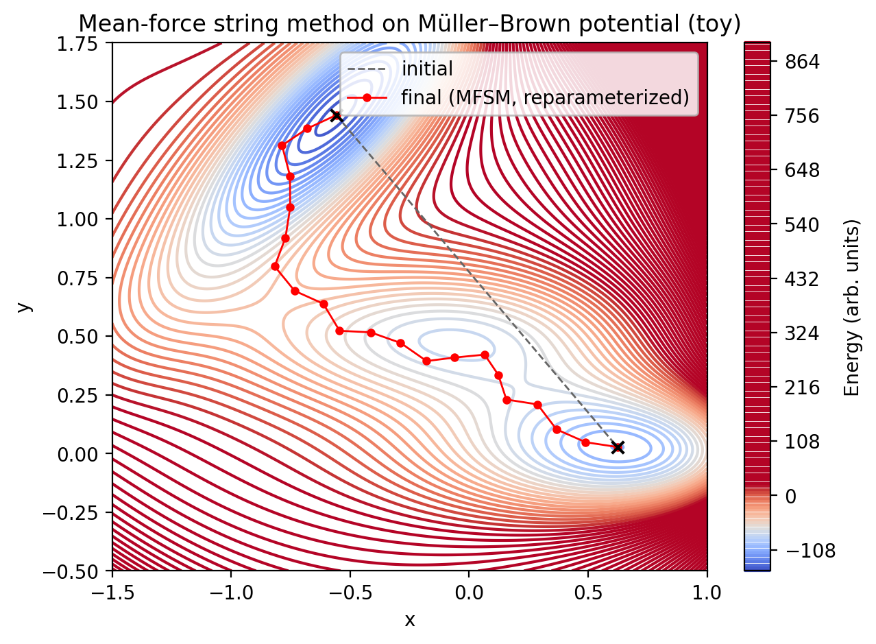
Choose two endpoints (near two minima) and initialize an initial string by linear interpolation (≈21 images).
Iterate (mean-force string method idea):
1. For each image $\phi_i$, run restrained sampling (harmonic umbrella centered at $\phi_i$).
2. Estimate the mean force using the umbrella identity:
  \[\mathbf{F}(\phi_i) \equiv -\nabla F(\phi_i) \approx \kappa \left(\langle \mathbf{x} \rangle_{\text{bias}} - \phi_i\right)\]
3. Project the force perpendicular to the local string tangent and update the image:
  \[\mathbf{F}_{\perp}(\phi_i) = \mathbf{F}(\phi_i) - \bigl(\mathbf{F}(\phi_i)\cdot \hat{\mathbf{t}}_i\bigr)\,\hat{\mathbf{t}}_i\]
  where a common choice for the unit tangent is
  \[\hat{\mathbf{t}}_i = \frac{\phi_{i+1}-\phi_{i-1}}{\lVert \phi_{i+1}-\phi_{i-1}\rVert}.\]
4. Reparameterize the string so images remain uniformly spaced in arc length.
5. Keep endpoints fixed (at least the first bead).

Run it

tutorials/string_method/string_method_test.py

python tutorials/string_method/string_method_test.py

It writes the following outputs:

Potential-only plots:
- tutorials/string_method/muller_brown_contour.png
Langevin demo:
- tutorials/string_method/langevin_trajectory_1000_steps.gif
Mean-force string method:
- tutorials/string_method/string_method_path.png (initial vs final reparameterized string)
- tutorials/string_method/string_method_path.gif (string evolution over iterations; first bead held fixed)
PMF:
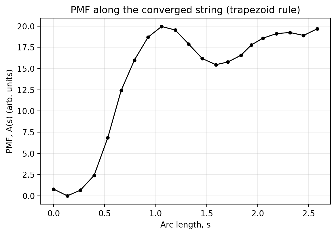
- tutorials/string_method/pmf_along_string.png (PMF along the converged string via trapezoid rule)

Quick preview (these files are generated by the script above):

Mean-force string method iterations (toy) — Toy mean-force string method on the Müller–Brown potential (endpoints fixed).

Initial and final (reparameterized) string path on the Müller–Brown potential — Initial string (gray) vs final reparameterized string (red) after the last iteration (uniform arc-length spacing of beads).

Parameters

The script uses overdamped Langevin sampling and adds mean-force string-method hyperparameters (see __main__ in tutorials/string_method/string_method_test.py):

Symbol	Meaning	Script value (default)
`dt`	Langevin timestep	`5e-4`
`kappa`	restraint strength	`200`
`dtau`	string update step	`0.01`
`n_images`	number of beads	`21`
`n_replicas`	replicas per bead	`4`
`n_equil`	equilibration steps per bead/replica	`150`
`n_samples`	sampling steps per bead/replica	`300`
`stride`	sampling stride	`2`
`max_step`	max bead displacement per iteration	`0.10`
`n_iters`	iterations	`100`

Reparameterization (uniform arc length)

Reparameterization is the “keep the beads evenly spaced” step. This demo does this by:

Computing cumulative distances along the polyline, then normalizing to $[0,1]$.
Linearly interpolating $(x(s), y(s))$ back onto a uniform $s$ grid.

The script implements the same idea (see reparameterize() in tutorials/string_method/string_method_test.py).

PMF along the string (trapezoid rule)

Once you have a converged string ${\phi_i}_{i=0}^{N-1}$ and an estimate of the mean force at each image $\mathbf{F}(\phi_i)\equiv -\nabla A(\phi_i)$, you can compute a 1D PMF along the path by integrating the tangential component of the force.

Define an arc-length coordinate

\[s_0=0,\qquad s_i=\sum_{k=1}^{i}\lVert \phi_k-\phi_{k-1}\rVert,\qquad \Delta s_i = s_{i+1}-s_i = \lVert \phi_{i+1}-\phi_i\rVert.\]

Let $\hat{\mathbf t}i$ be the unit tangent at image $i$ (e.g. $\hat{\mathbf t}_i \propto \phi{i+1}-\phi_{i-1}$), and define

\[F_{\parallel,i} = \mathbf{F}(\phi_i)\cdot \hat{\mathbf t}_i.\]

Then the PMF difference along the string is the line integral

\[A(s) - A(0) = -\int_0^{s} F_{\parallel}(s')\,ds',\]

and with discrete images you can approximate it with the trapezoid rule:

\[A_{i+1} \approx A_i - \frac{1}{2}\bigl(F_{\parallel,i}+F_{\parallel,i+1}\bigr)\,\Delta s_i.\]

In practice you typically set $A_0=0$ and report a relative PMF (you can also shift by A -= A.min() for plotting).

Minimal Python snippet

import numpy as np

# images: (N, d) array of string beads  phi_i
# F:      (N, d) array of mean forces  F(phi_i) = -∇A(phi_i)
phi = np.asarray(images, dtype=float)
F = np.asarray(mean_forces, dtype=float)

ds = np.linalg.norm(np.diff(phi, axis=0), axis=1)
s = np.concatenate([[0.0], np.cumsum(ds)])

# unit tangents
t = np.zeros_like(phi)
t[0] = phi[1] - phi[0]
t[-1] = phi[-1] - phi[-2]
t[1:-1] = phi[2:] - phi[:-2]
t_hat = t / (np.linalg.norm(t, axis=1, keepdims=True) + 1e-12)

F_par = np.sum(F * t_hat, axis=1)
dA = -0.5 * (F_par[:-1] + F_par[1:]) * ds
A = np.concatenate([[0.0], np.cumsum(dA)])

Example PMF along the converged string computed by trapezoid integration of the tangential mean force.

Notes

This script is a toy demonstration on a 2D potential, meant to illustrate the workflow. For real MFEP calculations you typically replace the “toy restrained dynamics” step with properly converged restrained sampling in your CVs (and update images using mean forces projected normal to the string).
In production string-method runs, you usually hold endpoints fixed in the metastable basins.

How do we use it in real systems/MD integrators?

The only essential requirement is the ability to run sampling with a harmonic bias on your chosen CVs (an umbrella potential). Practically every MD package supports this (directly, or via CV tooling like PLUMED/Colvars).

A common workflow looks like:

Define endpoints (structures or ensembles A and B) and pick CVs that separate them.
Generate an initial guess path between A and B (often via steered MD / targeted MD / a morph in CV space).
Initialize the string by placing $N$ images along that guess (e.g., by interpolation in CV space).
For each image, run an umbrella window with bias
\[U_{\mathrm{bias}}(\mathbf{z}) = \frac{\kappa}{2}\,\lVert \mathbf{z}-\phi_i\rVert^2,\]
then estimate the mean force at $\phi_i$ from the restrained ensemble (as in the earlier section).
Update images (typically using the force component perpendicular to the string), reparameterize, keep endpoints fixed, and iterate to convergence.

The elegance is that the per-image windows are independent: you can run all restrained simulations in parallel, then do a lightweight “string update” step between iterations.