Computing Fractional Membrane Potential

📋 Tutorial Summary
Learn how to compute the fractional membrane potential from PMEpot output. This method separates voltage-dependent contributions from the reaction-field potential, enabling quantitative analysis of transmembrane electric fields in MD simulations.

Overview

This tutorial walks through generating the fractional membrane potential of a planar membrane system. We cover:

1. The underlying theory (linear-response decomposition)
2. Setting up NAMD simulations with applied electric fields
3. Computing PMEpot maps in VMD
4. Post-processing to extract the membrane potential

Inputs

Download example data: a tarball containing step5_input.psf, pos.dcd, and neg.dcd (positve and negative voltage trajectories) is available: https://drive.google.com/file/d/1IN766-hRTBPqVSkxA3XaqkwAfwDf1dau/view?usp=sharing

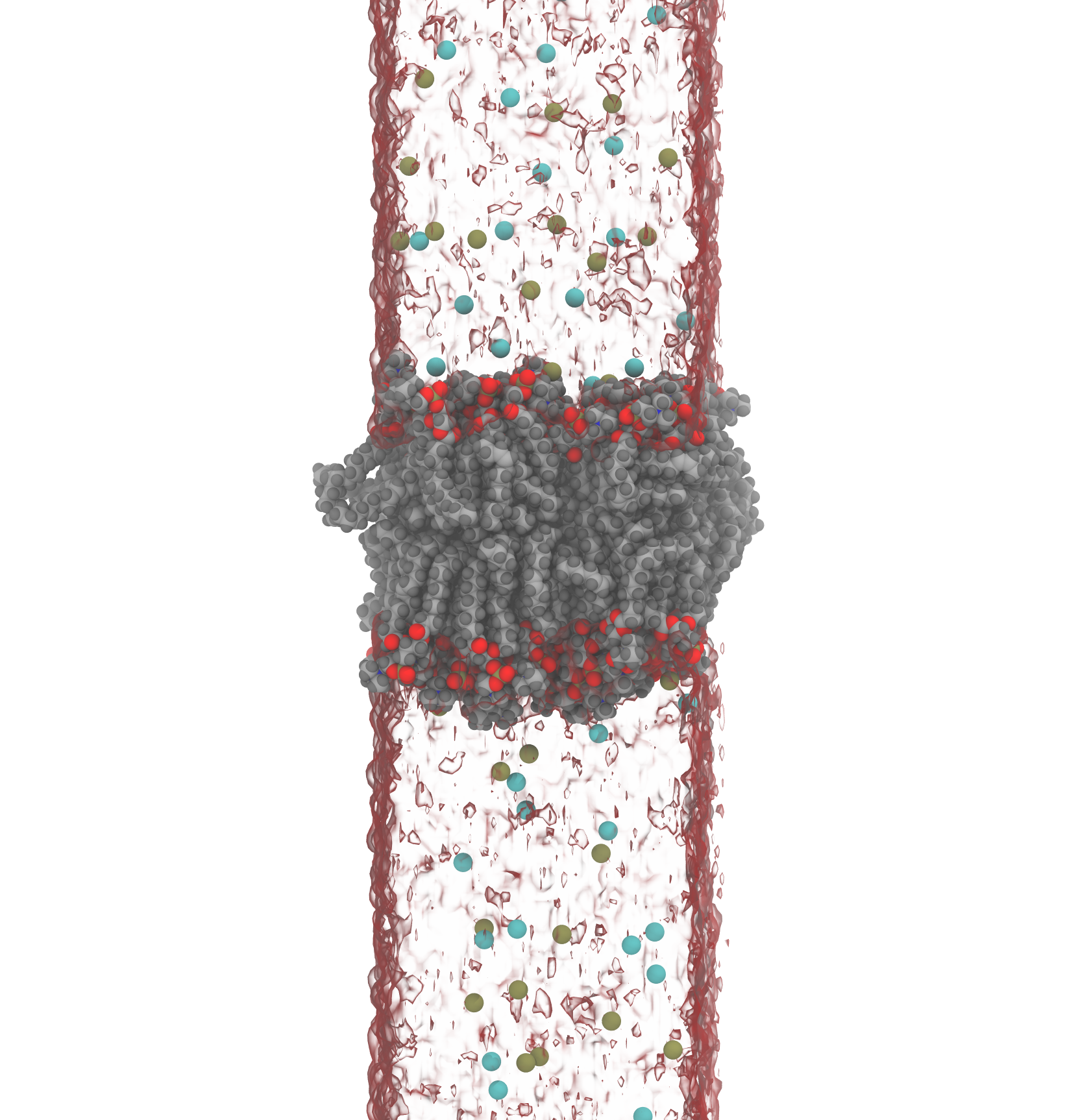
Toy system

Background

Biological membranes are essentially electrical circuits. The same physics from introductory electromagnetism applies—and this perspective lets us study membrane proteins quantitatively. Electrophysiology experiments measure ionic conductance through membranes; we can compute analogous quantities in silico using methods developed since the 1990s.

This tutorial uses linear-response theory to generate a membrane potential map.

📚 Suggested Reading

Key References

1. Roux, B. “Influence of the membrane potential on the free energy of an intrinsic protein.”
   Biophys. J. 73, 2980–2989 (1997). PMC1181204

2. Roux, B. “The membrane potential and its representation by a constant electric field in computer simulations.”
   Biophys. J. 95, 4205–4216 (2008). PMC2567939

A brief review of the theory is presented below. The solution of the linearized Poisson–Boltzmann equation developed by Roux (1997) shows that the total electrostatic potential can be decomposed as

In simple terms, this expression states that the total electrostatic potential $\phi_{\mathrm{tot}}(\mathbf{r};V)$ at position $\mathbf{r}$ in the presence of a transmembrane voltage $V$ can be written as the sum of two contributions. The first term, $\phi_{\mathrm{rf}}(\mathbf{r})$, is the reaction-field potential, which arises from the protein’s fixed charges together with the polarization and ionic screening of the surrounding environment in the absence of an applied voltage. The second term describes the effect of the applied membrane voltage: $\phi_{\mathrm{mp}}(\mathbf{r})$ is a dimensionless function that represents the fraction of the membrane potential experienced at position $\mathbf{r}$, so that multiplying it by $V$ gives the voltage-dependent contribution to the electrostatic potential.

Now, using the previous linearized equation, we extend it to the use of PMEpot and the external field. If we take two simulations at opposite voltages, we can isolate the voltage-dependent part (central difference):

and

Combining them gives:

Now solving for $\phi_{\mathrm{mp}}$ gives:

Implementation

We now implement this using molecular dynamics. This tutorial uses NAMD with the eField keyword, but most MD packages support applied electric fields.

⚠️ Use NVT, not NPT
NPT ensembles with external fields can introduce artifacts in the box dimensions. Run production with NVT for reliable membrane potential calculations.

Setting a Transmembrane Voltage in NAMD

To simulate a specific voltage across your simulation box (e.g., a transmembrane potential), you must apply a constant electric field. NAMD uses specific internal units, so you cannot simply enter the voltage in Volts.

1. The NAMD Configuration

Add the following lines to your production script (.inp):

eField on
eField 0 0 {EZ_Value}

Where {EZ_Value} is the electric field vector component in the Z-direction.

2. Calculating {EZ_Value} using the 0.0434 Factor

A useful shortcut for this calculation is the direct unit equivalence:

1 Unit $\left(\frac{\text{kcal}}{\text{mol} \cdot \text{Å} \cdot e}\right)$ is equivalent to $0.0434\,\text{V}/\text{Å}$.

Using this equivalence, the formula becomes:

Where:

• $V_{\text{target}}$ is the voltage in Volts.
• $L_z$ is the box length in Angstroms (Å).
• $0.0434$ is the conversion factor representing $\text{V}/\text{Å}$ per NAMD unit.

Example Calculation: +90 mV

Scenario: You want +90 mV across a box length ($L_z$) of $100~\text{Å}$.

💡 Tip: Find the box size in the .xsc file—the c_z column gives $L_z$:

# NAMD extended system configuration output file
#$LABELS step a_x a_y a_z b_x b_y b_z c_x c_y c_z o_x o_y o_z

1. Convert to Volts:

1. Calculate Electric Field in V/Å:

1. Convert to the NAMD Units:

Divide by the equivalence factor ($0.0434$):

1. Resulting Input:

eField on
eField 0 0 0.02074

📝 Note on the constant
The factor $0.0434$ is the inverse of the thermodynamic conversion: $1\,\text{eV} \approx 23.06\,\text{kcal/mol}$.

Restraints for PMEPot Analysis

⚠️ Important for membrane proteins
Apply position restraints to protein backbone atoms during the sampling window.

PMEpot averages the potential over multiple frames. If the protein translates or rotates, the resulting map will be spatially “smeared” relative to the fixed grid. Restraining the backbone keeps the protein aligned and prevents motion artifacts.

Computing the Electrostatic Potential with VMD

Once trajectories are complete, compute PMEpot maps in VMD. For reproducibility, run a Tcl script rather than using the GUI.

Run the Analysis

python tutorials/planer_membrane/pme_pot_figure.py

Headless mode (no GUI windows):

MPLBACKEND=Agg python tutorials/planer_membrane/pme_pot_figure.py

Script source: https://github.com/immunoguerrabulin/immunoguerrabulin.github.io/blob/main/tutorials/planer_membrane/pme_pot_figure.py

What the Script Computes

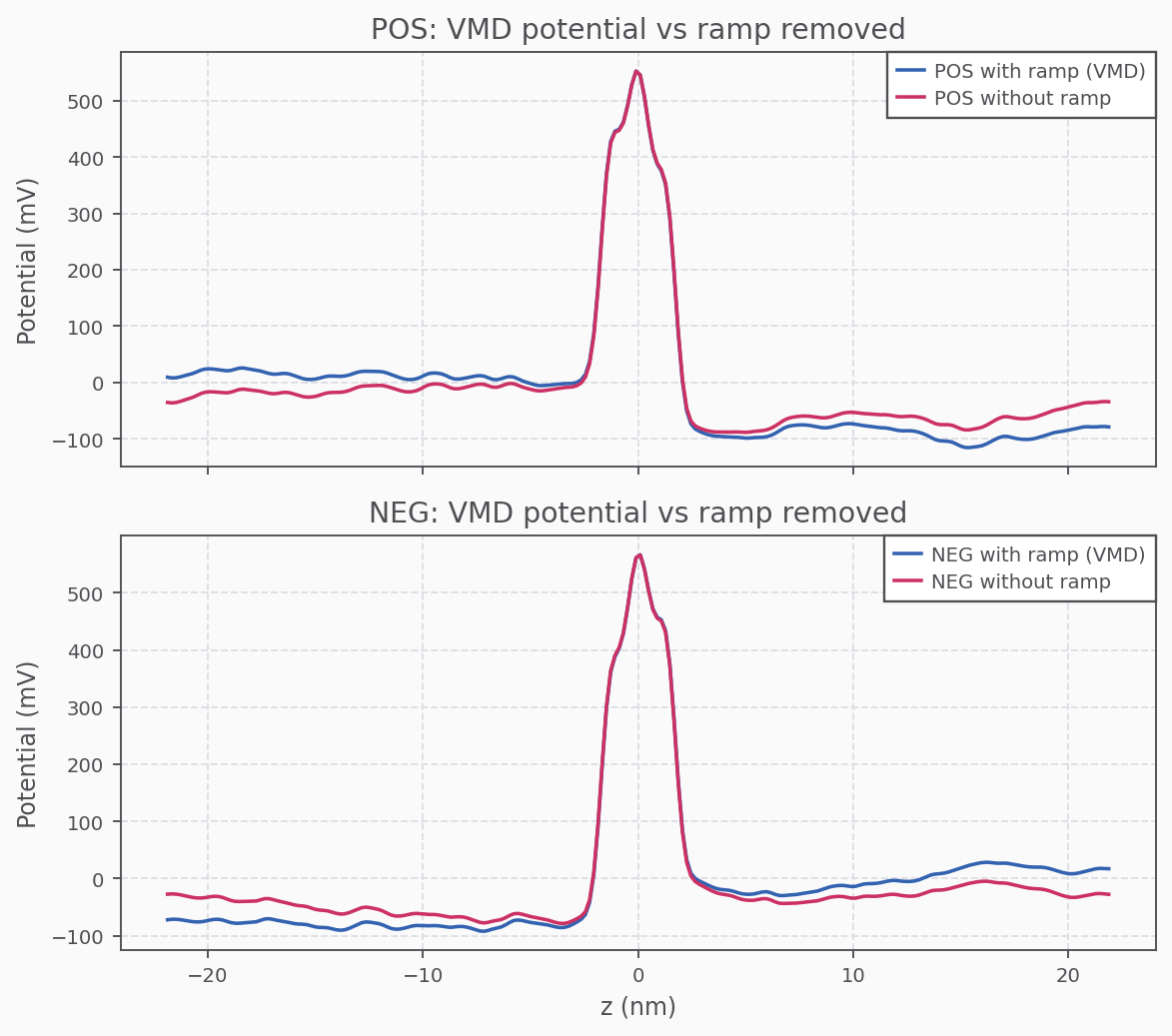
1. Adds the linear field ramp back to the VMD PMEpot output (VMD outputs molecular potentials without the applied field)
2. Builds z-profiles (XY-averaged) for both with-ramp and no-ramp potentials
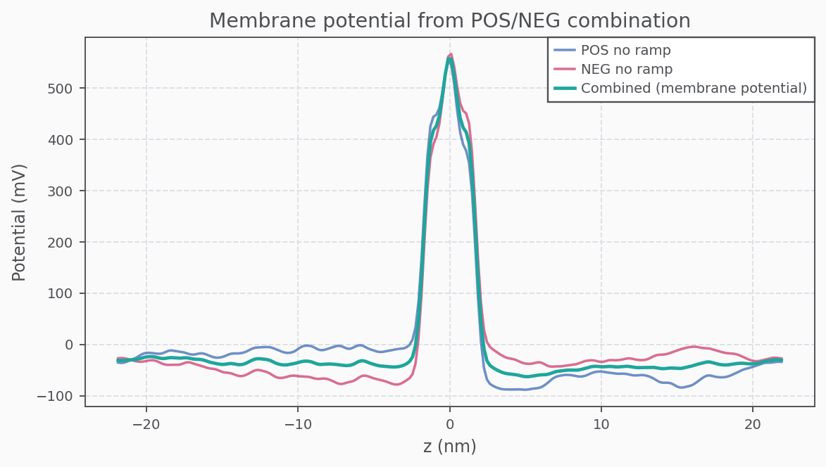
3. Combines POS/NEG into a single membrane-potential profile
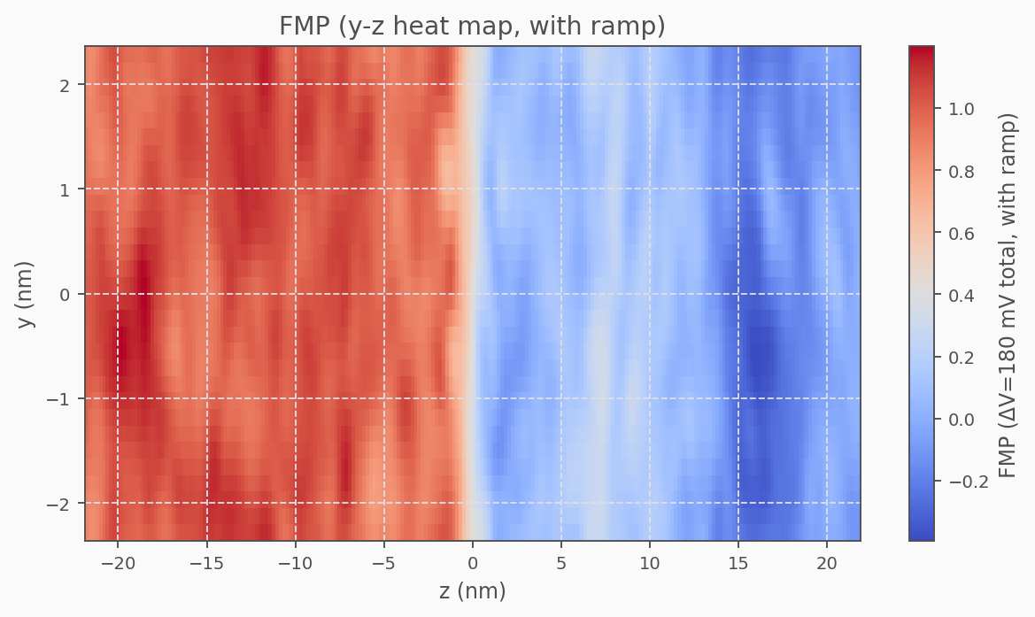
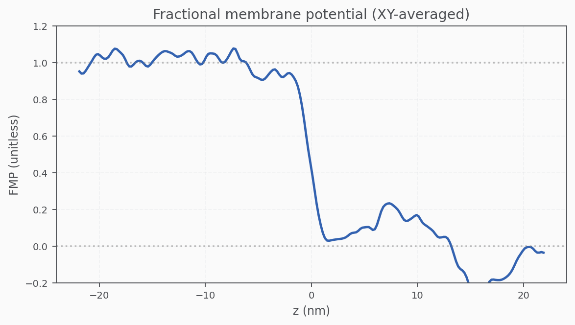
4. Computes fractional membrane potential (FMP):
   $\text{FMP} = \frac{\phi_{+V} - \phi_{-V}}{2\Delta V} + 0.5$

Output Files

Results

Ramp Removal (POS/NEG z-profiles)

Membrane Potential (Combined POS/NEG)

Fractional Membrane Potential (FMP)

Validation

The fractional membrane potential should be flat in bulk and linear across the membrane.

Comparison with Theory

Compare our 1D result to the analytic Poisson–Boltzmann solution from Roux (2008):

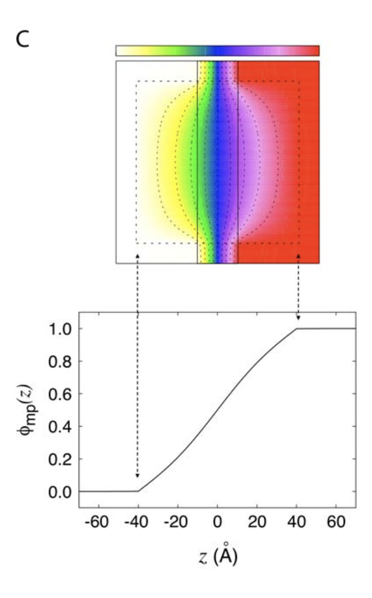
Good agreement! The MD-derived FMP reproduces the expected behavior from continuum electrostatics. There are some deviations from noise that can be solved by running the simulation longer.