Gillespie SSA for Stochastic Chemical Kinetics

📋 Tutorial Summary
Implement the Gillespie Stochastic Simulation Algorithm (SSA) to generate exact sample trajectories of reaction networks, then compute basic statistics from the ensembles.

Overview

The Gillespie Stochastic Simulation Algorithm (SSA) simulates a continuous-time Markov jump process by repeatedly sampling:

The time to the next reaction and
Which reaction happens next,

using the current propensities (reaction rates given the current state).

The original 1977 paper by Gillespie (link:https://pubs.acs.org/doi/10.1021/j100540a008) presents an excellent overview of the limitations of a purely deterministic approach to chemical kinetics. Gillespie argues for stochastic simulation methods because chemical reactions are inherently discrete and random. For example, molecular counts change by integer amounts and reaction events occur with probabilistic timing (think of Poission Distributions), producing stochastic fluctuations. The arguments in the paper are well reasoned and I highly recommend reading it. I would emphasize that stochastic simulations make the fluctuations (noise) of a model explicit, this is important for applications such as noise analysis of ion channels, which may be explored in a later tutorial.

This tutorial assumes knowledge of Monte Carlo simulations, and stochastic/transition matricies (Markov chain).

Some of this was adapted from a guest lecture I gave for “Simulation, Modeling, and Computation in Biophysics”.

Algorithm (the direct method)

The original paper uses different notation than I will present below. Figure 2 from Gillespie (1977) is quite clear, but from a pedagogical standpoint I find the transition-matrix explanation more convenient.

Using the $Q$-matrix (transition-rate matrix or infinitesimal generator) is the standard way to describe Markov chains (MCs). It makes the notation cleaner because the matrix explicitly defines both the holding time (diagonal elements) and the jump rates (off-diagonal elements).

Let $Q$ be the transition rate matrix where $Q_{ij}$ is the rate of moving from state $i$ to $j$, and the diagonal is the negative sum of all leaving rates:

\[Q_{ii} = -\sum_{j \neq i} Q_{ij}.\]

At current state $x$ (row index of $Q$) and time $t$:

Identify total exit rate ($a_0$): retrieve the diagonal element for the current state.
\[a_0 = -Q_{xx}\]
(Note: rate of leaving the state, $-Q_{xx} = k_{\text{forward}} + k_{\text{backward}}$.)
(Optional) Check stop condition: if $a_0 = 0$, the system is in an absorbing state. Stop.
Generate random numbers: draw $r_1, r_2 \sim U(0,1)$.
Compute time step ($\tau$): calculate the holding time using the total exit rate.
\[\\tau = \frac{-\ln(r_1)}{-Q_{xx}}\]
Determine transition move: use the off-diagonal elements to compute the probability of the forward jump.
\[p_{\text{fwd}} = \frac{Q_{x, x+1}}{-Q_{xx}}\]
If $r_2 < p_{\text{fwd}}$: set next state $x_{\text{next}} = x + 1$ (forward). Otherwise set $x_{\text{next}} = x - 1$ (backward).
Update:
\[t \leftarrow t + \tau\] \[x \leftarrow x_{\text{next}}\]

As a challenge, it is worth trying to code this yourself in your favorite language.

Let’s model the following system:

\[A \rightleftarrows B \rightleftarrows C\]

with rate constants (in $\mathrm{s}^{-1}$):

$k_{1f} = 5$, $k_{1b} = 2$
$k_{2f} = 10$, $k_{2b} = 4$
$k_{3f} = 20$, $k_{3b} = 1$

The python code is provided here:

Python example that uses a Q matrix

import numpy as np
import matplotlib.pyplot as plt
from collections import defaultdict
from pathlib import Path

def gillespie_from_Q(Q: np.ndarray, n_steps: int = 100_000, warmup: int = 0):
    Q = np.asarray(Q, dtype=float)
    if Q.ndim != 2 or Q.shape[0] != Q.shape[1]:
        raise ValueError("Q must be a square matrix")
    N = Q.shape[0]
    state = 0
    net = 0
    t_obs = 0.0
    t_total = 0.0
    traj = [(t_total, state)]
    for step in range(n_steps):
        a0 = -Q[state, state]
        if a0 <= 0.0:
            break
        dt = np.random.exponential(1.0 / a0)
        t_total += dt
        probs = Q[state].copy()
        probs[state] = 0.0
        probs = probs / a0
        r = np.random.random()
        cum = 0.0
        next_state = state
        for j in range(N):
            cum += probs[j]
            if r < cum:
                next_state = j
                break
        forward_event = ((next_state - state) % N) == 1
        state = next_state
        if step >= warmup:
            net += 1 if forward_event else -1
            t_obs += dt
            traj.append((t_total, state))
    flux = net / (t_obs * N) if t_obs > 0 else np.nan
    return flux, net, t_obs, traj

# Example: three-state chain A <-> B <-> C
kf = np.array([10.0, 10.0, 20.0])
kb = np.array([2.0, 5.0, 20.0])
N = 3
Q = np.zeros((N, N), dtype=float)
for i in range(N):
    Q[i, (i + 1) % N] = kf[i]
    Q[i, (i - 1) % N] = kb[i]
for i in range(N):
    Q[i, i] = -np.sum(Q[i])

flux_Q, net_Q, t_obs_Q, traj = gillespie_from_Q(Q, n_steps=100, warmup=0)
print(f"(Q)    flux={flux_Q:.6g} (net={net_Q}, t_obs={t_obs_Q:.4g} s)")
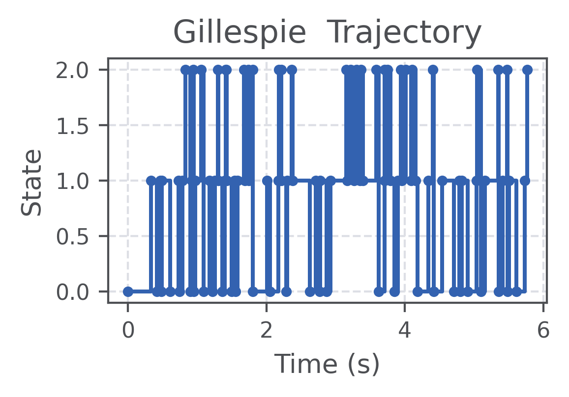
times, states = zip(*traj)
plt.step(times, states, where='post', marker='.', linestyle='-')
plt.xlabel("Time (s)")
plt.ylabel("State")
plt.title("Gillespie Trajectory")
out_path = Path("tutorials/gillespie-ssa/gillespie_trajectory.png")
out_path.parent.mkdir(parents=True, exist_ok=True)
plt.savefig(out_path, dpi=200, bbox_inches="tight")

# Longer simulation and empirical residence times
flux_Q, net_Q, t_obs_Q, traj_long = gillespie_from_Q(Q, n_steps=100000, warmup=0)
res_times = defaultdict(list)
if len(traj_long) >= 2:
    for (t0, s0), (t1, s1) in zip(traj_long[:-1], traj_long[1:]):
        res_times[s0].append(t1 - t0)

print('\nResidence time (empirical vs theoretical):')
for i in range(N):
    emp = float('nan')
    if len(res_times[i]) > 0:
        emp = np.mean(res_times[i])
    theo = 1.0 / (-Q[i, i]) if -Q[i, i] > 0 else float('nan')
    print(f" state {i}: emp={emp:.6g} s, theo={theo:.6g} s")

The output will look like:

(Q)    flux=1.50273 (net=26, t_obs=5.767 s)

Residence time (empirical vs theoretical):
 state 0: emp=0.0835453 s, theo=0.0833333 s
 state 1: emp=0.0669106 s, theo=0.0666667 s
 state 2: emp=0.0248728 s, theo=0.025 s

As a sanity check, for a two-state system the mean lifetime in a state is $1/(k_f + k_b)$; in the code above I estimate the mean lifetime from the simulated trajectory and compare it to the theoretical value. They agree!

Trajectory plot (saved by the code above):

Next steps

This tutorial provides a quick example of stochastic simulation using the Gillespie algorithm. These methods are widely used in biophysical modeling (ion channels and chemical reaction networks…) and deserve deeper treatment in a dedicated tutorial. One natural next step is to analyze the forward/backward switching in the trajectory as a noisy time series, for example by computing its power spectrum via a Fourier transform.